And also how – in the process – it shows the new RSSv4 TLT series to be wrong and the UAHv6 TLT series to be right.
For those of you who aren’t entirely up to date with the hypothetical idea of an “(anthropogenically) enhanced GHE” (the “AGW”) and its supposed mechanism for (CO2-driven) global warming, the general principle is fairly neatly summed up here:

Figure 1. From Held and Soden, 2000 (Fig.1, p.447).
I’ve modified this diagram below somewhat, so as to clarify even further the concept of “the raised ERL (Effective Radiating Level)” – referred to as Ze in the schematic above – and how it is meant to ‘drive’ warming within the Earth system; to simply bring the message of this fundamental premise of “AGW” thinking more clearly across.
First, we have the “no forcing” (t0) scenario, where Earth’s ‘effective emission’ to space comes from lower (and thus warmer) tropospheric layers:

Figure 2.
Then we have the “doubled CO2” (t1) scenario, where the ERL has been pushed higher up into cooler air layers closer to the tropopause:

Figure 3.
Raymond Pierrehumbert explains how this works:
An atmospheric greenhouse gas enables a planet to radiate at a temperature lower than the ground’s, if there is cold air aloft. It therefore causes the surface temperature in balance with a given amount of absorbed solar radiation [ASR] to be higher than would be the case if the atmosphere were transparent to IR. Adding more greenhouse gas to the atmosphere makes higher, more tenuous, formerly transparent portions of the atmosphere opaque to IR and thus increases the difference between the ground temperature and the radiating temperature. The result, once the system comes into equilibrium, is surface warming.
So when the atmosphere’s IR opacity increases with the excess input of CO2, the ERL is pushed up, and, with that, the temperature at ALL ALTITUDE-SPECIFIC LEVELS of the Earth system, from the surface (Ts) up through the troposphere (Ttropo) to the tropopause, directly connected via the so-called environmental lapse rate, i.e. the negative temperature profile rising up through the tropospheric column, is forced to do the same.
How, then, is this mechanism supposed to manifest itself?
Well, as the ERL, basically the “effective atmospheric layer of OUTWARD (upward) radiation”, the one conceptually/mathematically responsible for the All-Sky OLR flux at the ToA, and from now on, in this post, dubbed rather the EALOR, is lifted higher, into cooler layers of air, the diametrically opposite level, the “effective atmospheric layer of INWARD (downward) radiation” (EALIR), the one conceptually/mathematically responsible for the All-Sky DWLWIR ‘flux’ (or “the atmospheric back radiation”) to the surface, is simultaneously – and for the same physical reason, only inversely so – pulled down, into warmer layers of air closer to the surface. This latter concept was explained already in 1938 by G.S. Callendar:
When radiation takes place from a thick layer of gas, the average depth within that layer from which the radiation comes will depend upon the density of the gas. Thus if the density of the atmospheric carbon dioxide is altered it will alter the altitude from which the sky radiation of this gas originates. An increase of carbon dioxide will lower the mean radiation focus, and because the temperature is higher near the surface the radiation is increased, without allowing for any increased absorption by a greater total thickness of the gas.
Feldman et al., 2015, (as an example) confirm that this is still how “Mainstream Climate Science (MCS)” views this ‘phenomenon’:
Surface forcing represents a complementary, underutilized resource with which to quantify the effects of rising CO2 concentrations on downwelling longwave radiation. This quantity is distinct from stratosphere-adjusted radiative forcing at the tropopause, but both are fundamental measures of energy imbalance caused by well-mixed greenhouse gases.
The gist being that, when we make the atmosphere more opaque to IR by putting more CO2 into it, “the atmospheric back radiation” (all-sky DWLWIR at sfc) will naturally increase as a result, reducing the radiative heat loss (net LW) from the surface up. And do note, it will increase regardless of (and thus, on top of) any atmospheric rise in temperature, which would itself cause an increase. Which is to say that it will always distinctly increase also RELATIVE TO tropospheric temps (which are, by definition, altitude-specific (fixed at one particular level, like ‘the lower troposphere’ (LT))). That is, even when tropospheric temps do go up, the DWLWIR should be observed to increase systematically and significantly MORE than what we would expect from the temperature rise alone. Because the EALIR moves further down.
Conversely, at the other end, at the ToA, the EALOR moves the opposite way, up into colder layers of air, which means the all-sky OLR (the outward emission flux) should rather be observed to systematically and significantly decrease over time relative to tropospheric temps. If tropospheric temps were to go up, while the DWLWIR at the surface should be observed to go significantly more up, the OLR at the ToA should instead be observed to go significantly less up, because the warming of the troposphere would simply serve to offset the ‘cooling’ of the effective emission to space due to the rise of the EALOR into colder strata of air.
Which would lead us to expect the average OLR intensity level, if there weren’t also Earth system warming going on due to some other mechanism besides that of an “enhanced GHE”, like, say, an increase in solar heat input (+ASR), to stay relatively constant (flat) as tropospheric temps keep rising (the simultaneous effects of incrementally higher Ttropo and incrementally higher Ze effectively cancelling each other out), giving rise to an evident, gradual, yet ever-growing divergence between the two parameters. We see this basic expectation pointed out in the original caption of Fig.1 above, from Held and Soden, 2000: “Note that the effective emission temperature (Te) [after a doubling of atmospheric CO2] remains unchanged.”
Worth bearing in mind, however: We would expect to observe such gradual, ever-growing divergence between OLR and TLT in all cases, if there is in fact “GH enhancement” going on, not just in the basic case of no extrinsic warming (from, say, +ASR), i.e. flat OLR. If the OLR itself does go up, (due to e.g. solar warming), the TLT will simply end up rising faster and more (solar warming + “greenhouse warming”).
What we’re looking for, then, if indeed there is an “enhancement” of some “radiative GHE” going on in the Earth system, causing global warming, is ideally the following:
- OLR stays flat, while TLT increases significantly and systematically over time;
- TLT increases systematically over time, but DWLWIR increases even significantly more.
Effectively summed up in this simplified diagram:

Figure 4. Note, this schematic disregards – for the sake of simplicity – any solar warming at work.
However, we also expect to observe one more “greenhouse” signature.
If we expect the OLR at the ToA to stay relatively flat, but the DWLWIR at the sfc to increase significantly over time, even relative to tropospheric temps, then, if we were to compare the two (OLR and DWLWIR) directly, we’d, after all, naturally expect to see a fairly remarkable systematic rise in the latter over the former (refer to Fig.4 above).
Which means we now have our three ways to test the reality of an hypothesized “enhanced GHE” as a ‘driver’ (cause) of global warming.
The null hypothesis in this case would claim or predict that, if there is NO strenghtening “greenhouse mechanism” at work in the Earth system, we would observe:
- The general evolution (beyond short-term, non-thermal noise (like ENSO-related humidity and cloud anomalies or volcanic aerosol anomalies))* of the All-Sky OLR flux at the ToA to track that of Ttropo (e.g. TLT) over time;
- the general evolution of the All-Sky DWLWIR at the surface to track that of Ttropo (Ts + Ttropo, really) over time;
- the general evolution of the All-Sky OLR at the ToA and the All-Sky DWLWIR at the surface to track each other over time, barring short-term, non-thermal noise.
* (We see how the curve of the all-sky OLR flux at the ToA differs quite noticeably from the TLT and DWLWIR curves, especially during some of the larger thermal fluctuations (up or down), normally associated with particularly strong ENSO events. This is because there are factors other than pure mean tropospheric temperatures that affect Earth’s final emission flux to space, like the concentration and distribution (equator→poles, surface→tropopause/stratosphere) of clouds, water vapour and aerosols. These may (and do) all vary strongly in the short term, significantly disrupting the normal temperature↔flux (Stefan-Boltzmann) connection, but in the longer term, they display a remarkable tendency to even out, leaving the tropospheric temperature signal as the only real factor to consider when comparing the OLR with Ttropo (TLT). Or not. The “AGW” idea specifically contends, resting on the premise, that these other factors (and crucially also including CO2, of course) do NOT even out over time, but rather accrue in a positive (‘warming’) direction.)
The first point above we have already covered extensively. The combined ERBS+CERES OLR record is seen to track the general progression of the UAHv6 TLT series tightly, both in the tropics and near-globally, all the way from 1985 till today (the last ~33 years), as discussed at length both here and here.
Since, however, in this post we’re specifically considering the CERES era alone, this is how the global OLR matches against the global TLT since 2000:

Figure 5.
This is simply the monthly CERES OLR flux data properly scaled (x0.266), enabling us to compare it more directly to temperatures (W/m2→K), and superimposed on the UAH TLT data. Watch how closely the two curves track each other, beyond the obvious noise. To highlight this striking state of relative congruity, we remove the main sources of visual bias in Fig.5 above. Notice, then, how the red OLR curve, after the 4-year period of fairly large ENSO-events (La Niña-El Niño-La Niña) between 2007/2008 and 2011/2012, when the cyan TLT curve goes both much lower (during the flanking La Niñas) and much higher (during the central El Niño), quickly reestablishes itself right back on top of the TLT curve, just where it used to be prior to that intermediate stretch of strong ENSO influence. And as a result, there is NO gradual divergence whatsoever to be spotted between the mean levels of these two curves, from the beginning of 2000 to the end of 2015:

Figure 6.
This already quite definitive observation can still be further confirmed in a difference (“TLT residual”) plot:

Figure 7.
Yes, there’s a big lift there at the end, but there’s nothing ‘gradual’ or ‘systematic’ about it. In fact, it happens to occur – abruptly and precipitously – towards the end of 2015, right before the time when the 2015/2016 El Niño is about to top out. It is very easy in such a case for your eyes to fall victim to a so-called “end-point bias”, making you think you see a genuine overall divergence. But you don’t. The particular divergence that is inevitably drawing your eyes to it, started only right there, towards the end. If we simply remove it, the plot in Fig.7 would look like this:

Figure 8.
And poof! Gone is the sense of an upward incline …
Now, at this stage some might ask – and rightfully so – why I keep using the UAHv6 TLT dataset only in these comparisons. There are, after all, other tropospheric temperature datasets out there. Well, there is at least ONE very good reason why, and I will get to that soon enough, as it happens to be half the point of this entire post. In the meantime, please bear with me …
The second point above is just as relevant as the first one, if we want to confirm (or disconfirm) the reality of an “enhanced GHE” at work in the Earth system. We compare the tropospheric temperatures with the DWLWIRsfc ‘flux’, that is, the apparent atmospheric thermal emission to the surface:

Figure 9. Note how the scaling of the flux (W/m2) values is different close to the surface than at the ToA. Here at the DWLWIR level, down low, we divide by 5 (x0.2), while at the OLR level, up high, we divide by 3.76 (x0.266).
We once again observe a rather close match overall. At the very least, we can safely say that there is no evidence whatsoever of any gradual, systematic rise in DWLWIR over the TLT, going from 2000 to 2018. If we plot the difference between the two curves in Fig.9 to obtain the “DWLWIR residual”, this fact becomes all the more evident:

Figure 10.
Remember now how the idea of an “enhanced GHE” requires the DWLWIR to rise significantly more than Ttropo (TLT) over time, and that its “null hypothesis” therefore postulates that such a rise should NOT be seen. Well, do we see such a rise in the plot above? Nope. Not at all. Which fits in perfectly with the impression we got at the ToA, where the TLT-curve was supposed to rise systematically up and away from the OLR-curve over time, but didn’t – no observed evidence there either of any “enhanced GHE” at work.
Let’s also, just for the fun of it (?), create a 60/40 compound Ts+Ttropo curve (60/40 in favour of the surface because the EALIR is hypothetically supposed to be situated ~1.5 km above the surface on average, while the weighted mean of the UAHv6 TLT measurements appears to lie at a level ~3.8 km above the surface, and so one could naturally infer that there should somehow be a sizeable surface signal apparent in the DWLWIR ‘flux’ as well) and compare that to the DWLWIR curve in Fig.9. This is how it would look:

Figure 11.
The overall correspondence certainly isn’t worse. (BTW, regarding the makeup of the green compound curve in Fig.11, here’s my “Real HadCRUt” surface series vs. UAHv6 TLT.)
Finally, the third point above is also pretty interesting. It is simply to verify whether or not the CERES EBAF Ed4 ‘radiation flux’ data products are indeed suggesting a strengthening of some radiatively defined “greenhouse mechanism”. We sort of know the answer to this already, though, from going through points 1 and 2 above. Since neither the OLR at the ToA nor the DWLWIR at the surface deviated meaningfully from the UAHv6 TLT series (the same one used to compare with both, after all), we expect rather by necessity that the two CERES ‘flux products’ also shouldn’t themselves deviate meaningfully overall from one another. And, unsurprisingly, they don’t:

Figure 12.
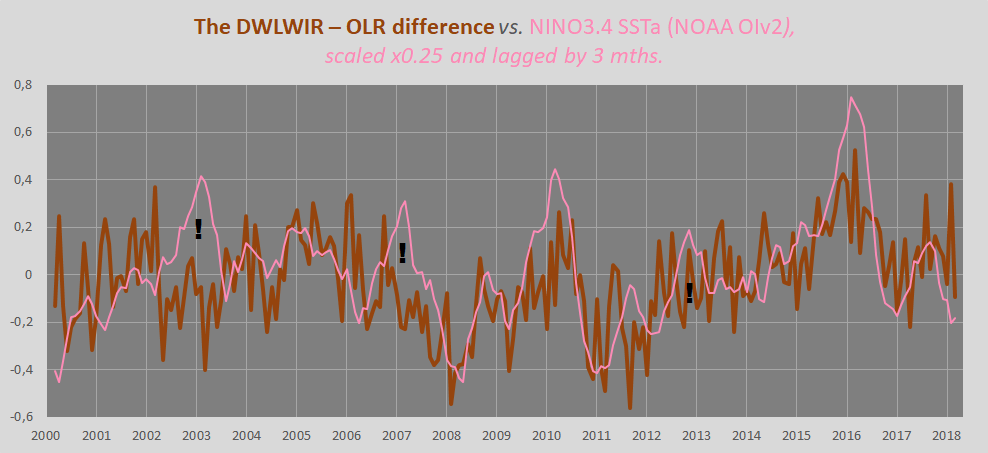
Difference plot (“DWLWIR residual”):
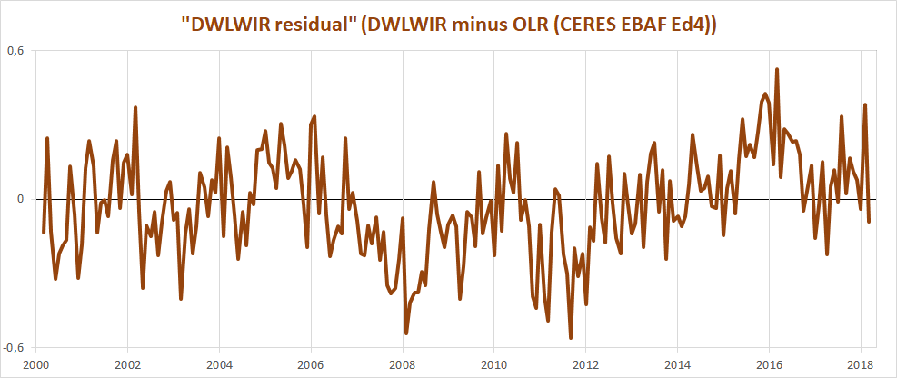
Figure 13.
Again, it is so easy here to allow oneself to be fooled by the visual impact of that late – obviously ENSO-related – peak, and, in this case, also a definite ENSO-based trough right at the start (you’ll plainly recognise it in Figs. 9, 11 and 12); another perfect example of how one’s perception and interpretation of a plot is directly affected by “the end-point bias”. Don’t be fooled:

Figure 14.
Remember what was pointed out early on upthread:
If we expect the OLR at the ToA to stay relatively flat, but the DWLWIR at the sfc to increase significantly over time, even relative to tropospheric temps, then, if we were to compare the two (OLR and DWLWIR) directly, we’d […] naturally expect to see a fairly remarkable systematic rise in the latter over the former (refer to Fig.4 above).
Looking at Figs. 12 and 14, and taking into account the various ENSO states along the way, does such a “remarkable systematic rise” in DWLWIR over OLR manifest itself during the CERES era?
I’m afraid not …
UAHv6 vs. RSSv4
In what way, then, does the CERES EBAF Ed4 data provide the evidence we need to confirm that the new RSSv4 TLT series is fundamentally flawed and that the UAHv6 TLT series is much closer to the truth, thus strongly supporting my decision to use the latter one as the sole representative of tropospheric temperatures (Ttropo) against the CERES ‘radiation flux’ data?
We’ve already put the UAHv6 TLT series to the test (in the above). We will now basically let the RSSv4 TLT series go through that same procedure.
What we need to do is simply to compare the TLT data with a) the All-Sky OLR at the ToA, and b) the All-Sky DWLWIR at the sfc, to check for internal consistency.
There are four options here:
- Your TLT series is correct, and the (radiatively defined) “GHE” is strengthening.
- Your TLT series is correct, and the “GHE” is not strengthening.
- Your TLT series is incorrect, and the “GHE” is strengthening.
- Your TLT series is incorrect, and the “GHE” is not strengthening.
For 1. to be the case, we need to observe your TLT series rising significantly and systematically relative to the all-sky OLR flux at the ToA, and at the same time the all-sky DWLWIR ‘flux’ to the sfc rising significantly and systematically relative to your TLT series.
For 2. to be the case, the OLR and DWLWIR should be observed to follow the same general course over time, no systematic divergence beyond natural noise, and your TLT series will be seen to track them both quite precisely over time.
For 3. to be the case, the DWLWIR should be observed to rise sharply over time relative to the OLR, but your TLT series won’t be seen to track between the two, as it should – rising systematically faster than the OLR, but more slowly than the DWLWIR.
For 4. to be the case, the OLR and DWLWIR should be observed to follow the same general course over time, but your TLT series won’t be seen to track either.
So what’s it gonna be?
We know from before that the general path taken by the UAHv6 TLT data between 2000 and 2018 matches impressively – and reassuringly – well with the general path taken by both the CERES EBAF Ed4 All-Sky OLR at the ToA data and the all-sky DWLWIR at the sfc data, thus lending strong support to two parallel ideas at once – that there is no observable strengthening of any radiatively defined “GHE” going on in the Earth system, and that the UAHv6 TLT series is more or less correct in its rendition of tropospheric temperature (Ttropo) evolution since the millennium. Scenario 2. above appears to be the one …
But what about the RSSv4 TLT data?
We first compare it with the all-sky OLR data, the radiative flux moving up and out of the Earth system to space through the top of the atmosphere (ToA):

Figure 15.
And the difference between the two curves in Fig.15 plotted:

Figure 16.
What do we see?
Even discounting those last 2+ years (from late 2015 to early 2018), we see a fairly obvious gradual and steady increase over time in TLT over OLR, from the relatively low average level of the first 4-5 years to the relatively high average level of the 3-4 years connecting the trough of the 2011/2012 La Niña and the peak of the 2015/2016 El Niño.
In other words, if the RSSv4 TLT series is correct, the two plots above are both clearly indicating a strengthening “greenhouse mechanism”, as radiatively defined, at work in the Earth system.
However, if this is indeed to be the case, there should also be an equally obvious radiative signature to be observed at the opposite end, down towards the surface. And here the situation should be inverted – TLT minus DWLWIR should slope systematically down, not up. Or, if we want to be consistent, comparing directly with the “DWLWIR residual” using the UAHv6 TLT series upthread, we would expect DWLWIR minus TLT to slope systematically up, which is basically saying the same thing, only the other way around.
Well, here’s RSSv4 TLT vs. CERES EBAF Ed4 All-Sky DWLWIR at the sfc:
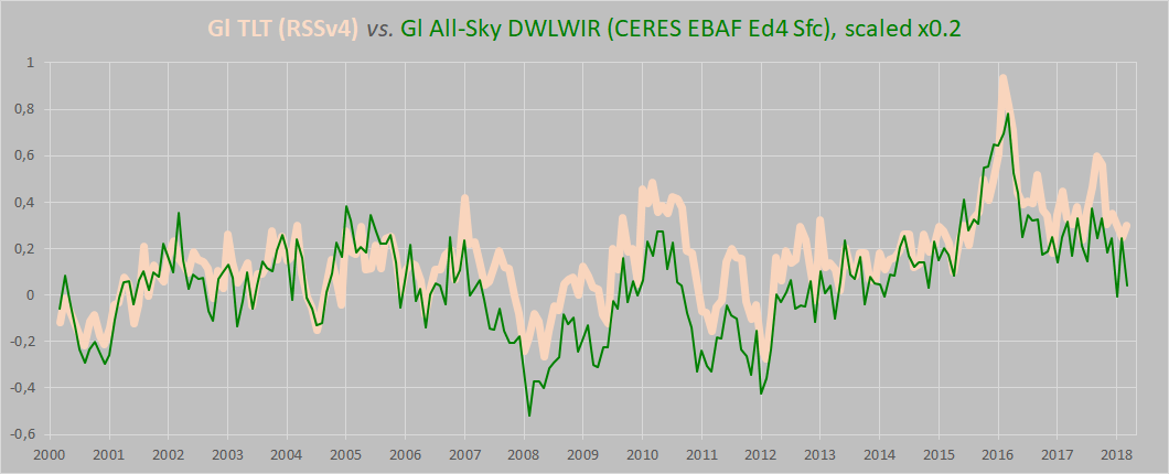
Figure 17.
And the difference plot to go along – DWLWIR minus TLT. Remember, according to “AGW theory”, it should go consistently and significantly UP:
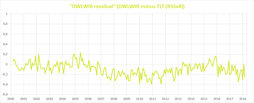
Figure 18.
Oops!
That’s the exact OPPOSITE of what we’d expect! If what was indicated in those ToA plots above were actually true. If the RSSv4 TLT series were actually correct.
There is no internal consistency to be found here …
IOW: The RSSv4 TLT series easily fails this simple test.
You can’t have it both ways. You can’t both have your TLT data increase significantly more over time than the ToA OLR data, and at the same time have it increase similarly more over time than the Sfc DWLWIR data. It makes absolutely no physical sense!
So, for the RSSv4 TLT series, scenario 4. above is the one that clearly portrays the real situation. Your TLT series is incorrect. (And there is no strengthening of a radiatively defined “GHE” going on in the Earth system.)

Hi Kristian,
Please derive the expression for calculating DWLWIR. The CERES data you use is model – derived, not observational.
I demonstrate DWLWIR=[(e+u-eu)P-eB+(1-e)(Q)]/(1-e), where e =1-(OLR/sigmaTs^4), u is the atmospheric short wave (solar insolation) emissivity, P is ASR, B is the radiative TOA imbalance, and Q is the non-radiative transfer of latent heat of evaporation plus sensible heat from the surface to the atmosphere. Does that sound right to you? Cheers.
PS. HIRS v02r07 now available! MAJOR changes compared to v02r02. Made me rewrite everything about my radiative model! It looks like ERBE + CERES now. I guess the two teams got together. A great improvement I must say, though it gives me some headache. Best regards.
Hi, Noegene Geo.
It is very much worth reading the data quality summary of the CERES EBAF-Surface Ed4 dataset:
Click to access CERES_EBAF-Surface_Ed4.0_DQS.pdf
It seems most relevant details are discussed there.
Actually, I came to a similar conclusion to yours, but via a different route. Over 1979 – 1992, an increased greenhouse effect caused all the surface warming. But over the period 1992 to 2017, all of the surface warming was caused by a decrease in albedo ( i.e. ASR increase), and there was no strengthening of the greenhouse effect. That’s what my model and HIRS v02r07, plus all the other data sets, tell me. Cheers.
I’m afraid we simply disagree on some of the fundamentals regarding this topic.
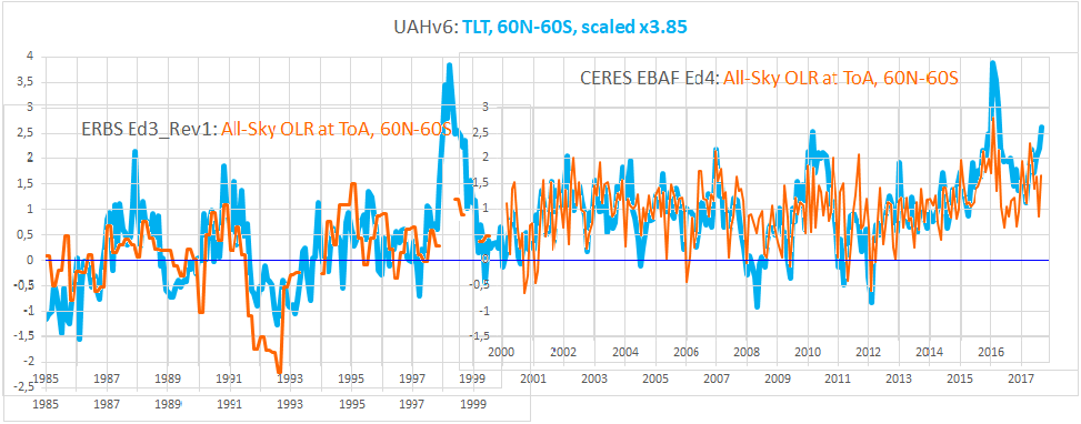
There was no “increased GHE” from 1979 to 1992. If your HIRS data tells you that, then it is wrong. I strongly suspect from what you’re saying that the obvious 1985 inhomogeneity calibration error seen in the HIRS data is still there:


There is no reduction in the All-Sky OLR at the ToA to be observed since 1985, from when the ERBS Ed3_Rev1 series begins. It simply follows the mean level TLT from then on. It also tracks TLT closely prior to the 1985 HIRS data gap. So why that abrupt, major step down from 1984 to 1986, right across the gap? Why there and nowhere else?
There is simply no good physical reason to explain it. That step is clearly just a methodological artefact.
Also worth taking into consideration: From 1979 to 1985, the period directly preceding the start of the ERBS+CERES record, there was no global warming at all:


The warming only started in 1988-1989, when the ASR began increasing. The ~12 years prior, Earth’s net heat balance very likely fluctuated around neutral – no net warming from neither ASR (+) nor OLR (–).
There is no evidence anywhere in the record of any ‘global warming’ produced by an “enhanced GHE”. All the warming we’ve seen is solar (from a decrease in albedo), evidently not as a secondary feedback effect (to warming), but distinctly as a primary cause.
Unfortunately the definition of the greenhouse effect here is complete rubbish. It is based on conservation of temperature. The law of physics that applies is conservation of energy. The same rubbish is applied to the belief that there is some ideal average temperature of the earth. But an average temperature is a meaningless quantity in thermodynamics. Unlike mass and length that can be added together to make a meaningful quantity, temperatures cannot be added together. The total temperature of two containers means nothing and so they cannot have an average that means anything. The same applies to the earth’s different climate zones.
I don’t quite understand why you use TLT. Are you using it as a proxy for surface temperature? If so, just compare the surface flux (generated from GHCN+ERSSTv5, use SB Law, weighted appropriately) to OLR, at least you then compare flux vs flux. Do you have something against the surface temperature data set? Yes, it is an approximation, but at least it is at the surface, unlike UAH-TLT. The ratio of surface flux to OLR is a proxy for the strength of the greenhouse effect. Do you agree?
I use TLT because OLR is more or less entirely a radiative expression and effect of tropospheric temps, not surface temps. You need to compare T_e to T_tropo to get it right. Whatever happens at the surface, it is never all radiative, so will confuse you as to what kind of mechanism caused what effect … That’s why you can’t conclude anything about the specifically radiatively defined strength of a “GHE” by just comparing T_s and T_e (that is, UWLWIR_s vs. all-sky OLR_toa).
And why would you compare a surface flux generated from GHCN+ERSSTv5 (with a terrible warming bias) when you already have the CERES EBAF Ed4 surface flux freely available?
A couple of points that confuse me.
EALIR should be considered the base of the atmosphere.
Your Figure 4 disregards changes in non-radiative transfers which have a big impact on DWLWIR.
Figure 4 also disregards the atmospheric window; 240 Wm-2 from ERL is not true.
A temperature minus a flux is not mathematically sound, as you used to determine your residuals.
I can see your point, you can express it much more clearly I am sure.
Neogene Geo,
All your points are completely beside the point. The idea of ‘global warming’ from an “enhanced GHE” relies fully on the basic premise of “All Else Being Equal”, meaning, nothing else changes as the initial radiative forcing starts working. We can only ever confidently expect it to work as hypothesized if this premise is true. And so your point about “changes in non-radiative transfers” is … pointless. Non-radiative transfers aren’t supposed to change other than as either negative or positive feedbacks to the “greenhouse” warming.
Fig.4 does not disregard the atmospheric window. The ERL is not an actual atmospheric layer, Neogene Geo. It is Earth’s CONCEPTUAL (mathematically defined) blackbody surface in space. Which means it hypothetically emits our planet’s ENTIRE thermal emission flux to space.
And I am not subtracting a flux from a temperature. I’ve translated the flux into a temperature (via the S-B equation) and only THEN subtract it from the other temperature …
Thanks for your replies Kristian.
I don’t know what you mean by “all else being equal”. I can equally track changes in ASR and atmospheric longwave emissivity with no constraints, and what their effect on surface flux is. Also, I just create the model and apply the data to it, I am not in the business of questioning the data supplied from the various sources, as I don’t have that expertise. So when Dr Lee produces an updated HIRS dataset, I must change my interpretation, whether I like it or no. By the way, I plotted GHCN+ERSSTv5 against the CERES surface LW flux, the influence of the first on the second is quite plain to see. Slightly different trends, but nothing too drastic.
I don’ t have any use for UAH TLT in my models, so we differ a lot in that respect.
Regards
Neogene Geo, you wrote:
Like I said, it simply means that nothing else – no other physical mechanisms or processes within the Earth system, such as evaporation and convection – changes as the initial radiative forcing from more CO2 in the atmosphere starts working. It is an ABSOLUTE requirement for the idea of ‘global warming’ from an “enhanced GHE” to work at all …
I wouldn’t either, unless I observe obvious signs of spurious changes when comparing those various data sources to other relevant sources, like in the case above.
Don’t use the HIRS dataset at all, is my advice. Use the ERBS+CERES dataset. That’s the authoritative one. That’s the gold standard, the benchmark series.
You should think this point through. We can not expect T_s to correlate directly with the radiative flux at the top of the atmosphere (ToA), the OLR (=> T_e), because the first one is influenced by radiative AND non-radiative processes, while the second one is a purely radiative effect (mostly of tropospheric temperatures). The connection between T_s and T_e is only secondary (indirect), and goes via the troposphere, in the way the surface affects tropospheric temps. Using T_s to assess the strength of a purely radiatively defined “GHE” will potentially end up garbling your results and conclusions …
Thanks for the reply. Interesting. I do however totally diagree about the connection between your Ts and Te. For my money, an energy budget comprises both radiative and non-radiative components (lets call them Q), and when I model them both into the overall budget, I find that Q contributes to DWLWIR, but not to surface flux nor OLR. That’s upcoming anyway.
Also, are you familiar with the DEEP-C project, and if so what do you make of their OLR reanalysis?
Best regards
Neogene Geo, you asked:
Yes, I am. That’s Richard P. Allan’s project. I discussed it at length here:
You even commented on that post …
Yes, but I didn’t immediately make the connection until I came across the Deep C database independently. I am still working on my model, now Read et al. 2016 has illustrated to me a very interesting “anti-greenhouse” effect on Mars during dust storms. My model can handle this, but I had not considered it as physically possible until now. Surface flux less than Te. Which is a bit of a wow for me. More later, I need to gather my thoughts and do more mathematical modelling. I have an end of January deadline for publication, and not enough time. Cheers.
That’s Read et al. Published in the Royal Meteorological Society Journal, to be clear. I liked this paper very much because of the way it summarises current understandings, and the secret to understanding Earth partly lies in understanding the other planets too. Cheers!
Only they don’t summarise the current understanding of Mars. They make the cardinal mistake of just uncritically quoting an old and terribly outdated theoretically based guesstimate of the global annual average T_s of Mars, specifically based ON the notion that there HAS to be some kind of “GHE” there too, given how much CO2 is in its atmosphere (stating (p.707, se link below)): “Hence, the Martian greenhouse warming is relatively modest, amounting to no more than around 5K at the surface (e.g. Pollack, 1979)”, and using a BB LW flux from the surface (123 W/m^2) translating into a T_s equal to ~216K). Problem is, though, that this theoretical guesstimate has never been backed up by real-world OBSERVATIONS of any kind. It is simply stated (and restated, ad nauseam) as an assumed “fact”. When it is no such thing.
T_e is considerably higher than T_s on Mars, Neogene Geo. This is based on actual temperature readings from globally orbiting satellites. I discussed this whole thing in this comment on another thread:
For the people wanting to read “Read et al., 2016,” for themselves, here’s a link:
Click to access Global%20energy%20budgets%20and%20trenberth%20diagrams%20for%20the%20climates%20of%20terrestrial%20and%20gas%20giant%20planets%202016.pdf
[…] recent article on the absence of “AGW warming” fingerprints in the CERES satellite data. How the CERES EBAF Ed4 data disconfirms “AGW” in 3 different ways by okulaer November 11, 2018. Excerpts below with my bolds. Kristian provides more detailed […]
[…] (okulaer) prefacing his analysis of “AGW warming” fingerprints in the CERES satellite data. How the CERES EBAF Ed4 data disconfirms “AGW” in 3 different ways by okulaer November 11, 2018. Excerpts below with my bolds. Kristian provides more detailed […]
[…] (okulaer) prefacing his analysis of “AGW warming” fingerprints in the CERES satellite data. How the CERES EBAF Ed4 data disconfirms “AGW” in 3 different ways by okulaer November 11, 2018. Excerpts below with my bolds. Kristian provides more detailed […]
Callendar’s observation that density determines focus (height) of back radiation, if true, should provide a simple to understand determination if there’s anything to CO2 causing global warming, no?
One can calculate for every barometric value the temp impact of each additional CO2 ppm.
If there’s no formula for Callendar’s point, the this could be determined experimentally, right?