Verifying my near-global 1985-2017 OLR record

---

It appears I was right 😎

33y TLT→OLR connection confirmed!

---

---

Turns out the results from my last blog post were challenged even before I published them. In a paper from 2014, Allan et al., the alii notably including principal investigator of the CERES team, Dr. Norman Loeb, went about reconstructing the ToA net balance (including the ASR and OLR contributing fluxes) from 1985 onwards, just like I did; in fact, it’s all right there in the title itself: “Changes in global net radiative imbalance 1985–2012”. I missed this paper completely, even when specifically managing to catch and discuss (in the supplementing post, Addendum I) its follow-up (Allan, 2017). The results and conclusions of Allan et al., 2014, regarding the downward (SW) and upward (LW) radiative fluxes at the ToA and how they’ve evolved since 1985, appear to disagree to a significant extent with mine. I was only very recently made aware of the existence of this paper, by a commenter on Dr. Roy Spencer’s blog, “Nate”, when he was kind enough to notify me (albeit in an ever so slightly hostile manner):

“What is stupid and cowardly is how Kristian refuses to confront the reality that the experts disagree with him about what we actually OBSERVE.

“Kristian, you have tried to draw conclusions from 33 y of data that you’ve stitched together by making various choices about offsets between the sets.

“But as I showed you, and you ignored, Loeb and collaborators have made different choices to produce a continuous set. And do not draw your conclusions.

“Here is a paper. (…)”

I thanked him for the link and went to have a look. I was curious, after all, and always up for a challenge. If there was indeed something I’d missed, some crucial observational datasets and/or interpretations that had passed me by and that would somehow change the whole picture, I was eager to find out about them. I was also very interested in reading about Allan et al.’s particular method of reconstruction and to assess their results based on it …

“Nate” seemed overly confident that this paper obliterates my entire argument – that there is no trace in 33 years of high-quality radiation flux data (ERBS+CERES) of an “enhanced GHE” contribution to ‘global warming’; that the data instead unequivocally shows that the Sun is behind it all; not –OLR accompanied by –ASR, as claimed/implied by “Mainstream Climate Science” (‘MCS’), but rather the opposite: +ASR accompanied by +OLR.

So, is “Nate” correct? Am I proven wrong?

Short answer: No.

However, the long answer is much more interesting, for it brings to light certain aspects of the obvious bias lying at the heart of the entire “Mainstream Climate Science (MCS)” endeavour and how it manifests itself in the analysis of climate data. The general thought process is so overwhelmingly controlled and constrained by the “AGW” idea, the reigning (and, in most people’s minds, undisputed and unchallenged) “climate paradigm” of our time, that more CO₂ in the atmosphere MUST cause (and IS causing) ‘global warming’, that people – SMART people! – don’t even think twice about it. They simply look past it. It is just taken as established fact. Gospel truth. Even when, in actuality, it is no such thing.

Well, I’ve been ranting about this silliness on this blog before, so I will stop here. And rather have a closer look at the paper at hand: Allan et al., 2014. Because it’s a good opportunity to delve a bit deeper into this matter.

---

So what is the issue? What is the bone of contention here?

First, here’s what I did …

To sum it up, I took two separate ToA radiation flux datasets (the ERBS Ed3_Rev1 and the CERES EBAF Ed4), spanning the 1985-1999 and 2000-2017 periods, respectively, and combined them into one full record, employing a tried and tested calibration procedure across the five-month 1999-2000 data gap between them. The starting point defined:

“We know what happens within those two consecutive timespans [1985-1999 & 2000-2017], covered by each radiation flux dataset [ERBS & CERES] separately and in succession. That’s really an open-and-shut case. The persisting pattern is unmistakable, undeniable.

“The only thing remaining, then, in order to settle this matter once and for all, is to find out what happens across the small (five-month) gap between our two radiation flux datasets. From Oct’99 to Feb’00. How do we merge them, stitch them together into one single record? How do we properly calibrate the one to the other?”

Referring to the following:

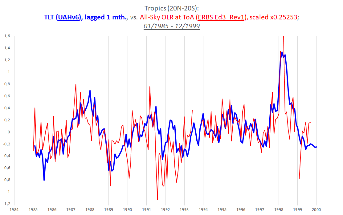
Figure 1. How the ToA radiation flux anomalies evolved within the 15-year ERBS period (1985-1999).

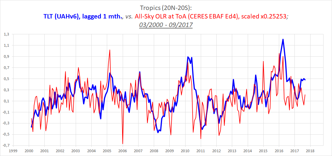
Figure 2. How the same ToA radiation flux anomalies have evolved within the 18-year CERES period (2000-2017).

We see that all fluxes, ASR (Q_in(SW)), OLR (Q_out(LW)) and Net alike, grow in intensity from start to finish within each separate period.

The only question, then, should really be what happens between these two periods? After all, that’s what will finally and ultimately settle the matter of whether an overall increase in ASR (from 1985 all the way to 2017) or an overall reduction in OLR (within the same time frame) is the cause behind our current positive Net flux (2012-2017) …

Within each segment it is obvious that the ASR and the OLR both increase, only with the increase in ASR larger in both cases, which in turn is the reason why the Net flux (ASR minus OLR) is also observed to increase in both cases, albeit much more distinctly within the first (ERBS) period.

And so it all seems pretty settled already. But it isn’t really. We have to find out what most likely happened across that 1999-2000 data gap between the ERBS and CERES datasets in order to be absolutely certain.

Here’s the three-step procedure allowing me, with a fair amount of confidence, to construct my calibrated composite 1985-2017 (ERBS+CERES) ToA flux record for the near-global (60N-60S):

1. I turned my focus on the OLR, noting how it appeared to track, to an impressive degree, tropospheric temps over time within each of the two separate periods (true both for the tropics (20N-20S) and for the near-global (60N-60S)), a circumstance which seems to make perfect sense, considering how the OLR should really for the most part simply be a radiative effect of tropospheric temps – the thermal emission flux of (primarily) Earth’s troposphere. My initial hypothesis – the first ‘guess’, so to say – then became, based on this very observation, that the OLR would also track the tropospheric temps across the 1999-2000 data gap. It’s a fair first step; seeing how the OLR and the TLT follow each other both during the 1985-1999 period (ERBS vs. UAH) and the 2000-2017 period (CERES vs. UAH), the assumption was made that the OLR and the TLT would also follow each other from 1999 to 2000, from the first half of the record to the second half.
   
   *1………………………………………………………………..*2
   
   *3………………………………………………………………..*4

   *1 T_e (OLR→; ERBS Ed3_Rev1) vs. T_tropo (TLT; UAHv6), 1985-1999, tropics.
   *2 T_e (OLR→; ERBS Ed3_Rev1) vs. T_tropo (TLT; UAHv6), 1985-1999, near-global;
   …..OLR: 72d avg., 10°×10°; TLT: monthly avg., 2.50°×2.50°.
   *3 T_e (OLR→; CERES EBAF Ed4) vs. T_tropo (TLT; UAHv6), 2000-2017, tropics.
   *4 T_e (OLR→; CERES EBAF Ed4) vs. T_tropo (TLT; UAHv6), 2000-2017, near-global;
   …..OLR: monthly avg., 1°×1°; TLT: monthly avg., 2.50°×2.50°.

2. This initial hypothesis was then made ready to be put to the test. I combined the two separate OLR curves (ERBS and CERES) into one by placing them on top of the single TLT curve (UAHv6), adjusting them in such a way and to such an extent that they matched the overall progression of the TLT curve from 1985 all the way to 2017. Now, keep in mind that doing this is not (!) itself proof that the match is real. I did the adjusting. To make it all match. The resulting combined OLR series (really, the offset between the ERBS and the CERES data) had yet to be confirmed. At this stage, it did nothing but visualise the prediction of my hypothesis, that the OLR would also follow the TLT across the 1999-2000 data gap. The particular hypothesis whose validity I was going to test. And I ended up testing it against other, independent radiation flux datasets with the particular utility of actually spanning the 1999-2000 ERBS-CERES data gap, like the ‘ISCCP FD’ and the ‘HIRS’ datasets (Step 3, below).
   
   *5………………………………………………………………..*6
   
   *7

   *5 T_e (OLR→; ERBS Ed3_Rev1+CERES EBAF Ed4) vs. T_tropo (TLT; UAHv6), 1985-2017, near-global; *2 and *4 combined.
   *6 T_e (OLR→; ERBS Ed3_Rev1+CERES EBAF Ed4) vs. T_tropo (TLT; UAHv6), 1985-2017, near-global; 6 mth. avg.
   *7 OLR (ERBS Ed3_Rev1+CERES EBAF Ed4), 1985-2017, near-global, with TLT-calibrated offset from *5.

3. Completing the test, I gained solid verification that the offset I had originally chosen was in fact more or less spot on. My prediction indubitably hit the mark. Which means my hypothesis stood firmly up to the test, adding greatly to the credibility of my composite OLR data record matching the overall progression of the TLT data from 1985 to 2017.

   
   *8…………………………………………………………*9

   *8 Testing the TLT-calibrated offset in OLR between the ERBS and CERES datasets in *5 and *7 against ISCCP FD.
   *9 Testing the TLT-calibrated offset in OLR between the ERBS and CERES datasets in *5 and *7 against HIRS.

But I would still consider this − the +0.92 W/m² offset at the 1999-2000 splice between the two separate observational datasets − to be the ‘weak link’ of my 1985-2017 composite OLR record. In fact, I’d expect this to be the only part that could realistically be ‘challenged’. Otherwise you would somehow have to find a way to challenge the validity of the contributing observational datasets themselves. On either side of my splice.

So, naturally, my initial question would be:

Does the 1985-2012 OLR reconstruction of Allan et al., 2014, somehow refute my 1999-2000 offset?

And the answer would be:

Not at all!

On the contrary, it soundly verifies it! Its final reconstructed OBS curve (the red one in their Fig.2b) matches more or less perfectly with mine across the 1999-2000 data gap (ERBS, 1994-1999, & CERES, 2000→). Which means that, rather than providing countering evidence suggesting my particular offset might after all be incorrect, it distinctly provides yet more independent evidence in direct support of it.

But, Allan et al.’s red OBS curve and my (yellow) composite curve do indeed disagree overall, don’t they? “Nate” is certainly not wrong in claiming that:

Figure 3. Left half shows (in red) Allan et al.’s final OBS OLR curve isolated, originally displayed in their Fig.2b superimposed on the model curves. Right half shows (in yellow) my composite (ERBS+CERES) near-global OLR record that I constructed in my “THE DATA:” post, and which can be seen also in Fig.*7 of this post. Both curves span the time interval 1985-2012 and are equally scaled.

No, he isn’t. What I’m saying is, Allan et al., 2014, and I do NOT disagree on the specific mean-level offset necessary between the ERBS and the CERES datasets across the data gap between them. [Which, as it happens, is the only thing that I’ve calibrated myself; the only thing about my full 1985-2017 composite record that I myself am personally and directly responsible for. The rest is just the official ERBS Ed3_Rev1 (Wong et al., 2006) and CERES EBAF Ed4 (Loeb et al., 2018) 60N-60S data. I’ve done nothing except plotting it.] On this, we agree completely …!

Figure 4. The two curves in Fig.3 compared directly, my yellow ERBS+CERES curve on top of Allan et al.’s OBS curve. The two blue vertical lines mark the specific data discontinuities that Allan et al. were interested in; the first one (1993-1994) within the ERBS dataset, the second one (1999-2000) between the ERBS and the CERES datasets (see below). [It is worth noting that the slight discrepancy observed post 2000 between the red and yellow curves (both CERES-based) stems from i) a difference in baseline periods (2001-2005, Allan et al.’s curve; 2005-2015, my curve), and ii) the fact that Allan et al. used EBAF Edition 2.7 data, while I use Edition 4.0 data; the two are not alike (Ed2.7 and Ed2.8 are virtually equal, according to the Ed2.8 Data Quality Summary).]

So where’s the actual discrepancy to be found? Well, it’s pretty plain to see, isn’t it? Across the 1993 ERBS data gap.

Which is to say that, in the end, what this paper all boils down to, is Allan et al. simply taking it upon themselves to arbitrarily (?) “correct” the ERBS Ed3_Rev1 dataset, as it seems, without even asking the people actually in charge of it what they might think, to create the impression that near-global all-sky OLR at the ToA did not increase in the least, but stayed completely flat overall (Fig.3, left panel), between 1985 and 2012, during a period of time when surface and tropospheric temps rose by ~0.3 °C, which should have resulted in a general increase in the OLR flux worth of about 1 W/m².

IF substantial strengthening of the “GHE” hadn’t been going on, that is …

Level OLR accompanied by rising T over time is, after all, what “we” (as in ‘MCS’) want to see. Because that’s theoretically the identifying mark of an “enhanced GHE” being the driver of the warming.

Accordingly, it is of course also what the models show:

Figure 5. Yellow curve: My composite observational 60N-60S all-sky OLR series (1985-1999: ERBS Ed3_Rev1, 72d avg.; 2000-2012: CERES EBAF Ed4, 3mth. moving avg.); blue curve: CMIP5 (rcp4.5) model mean 60N-60S ToA OLR (3mth. moving avg.); equal scales. [Observe how, using the original observational data from ERBS and CERES, plus the now (by Allan et al., 2014) reconfirmed 1999-2000 offset between the two, 60N-60S All-Sky OLR at the ToA (my yellow curve) is seen to easily make the temperature-required 1 W/m² rise in intensity from 1985 to 2012. The models, though, don’t agree. After all, according to “theory”, it really shouldn’t …]

You will note that the blue model mean tracks the yellow observations relatively well from 1994 (beyond the depths of the Pinatubo trench and the 1993 ERBS data gap) onwards, but not at all from 1985 to 1993.

[Keep in mind, when studying Fig.5 above, how the models tend to assume an unnaturally extended rebound period after large volcanic eruptions like El Chichón (1982) and Pinatubo (1991). It the latter case, it apparently took ten years after the original blast (all the way to mid 2001), according to the models, before the OLR level had managed to increase back and restabilised at the ‘zero level’. This, then, is the real reason why the blue model curve appears to agree so well with the yellow observations curve from 1994 to 2001. The observations curve does not rise out of the Pinatubo deep in the form of a slow rebound like the model curve does. It simply tracks the tropospheric temps (TLT), and rather shifts up in one step following the 1997/98 El Niño, just like they do. The flat post-Niño TLT trend (1998/99 →) is the reason why the mean level of the yellow OLR observations curve in Fig.5 stays flat as well. If the OLR had stayed flat because of an “enhanced GHE”, like the models assume, the TLT should – during the same time period – have gone markedly up. They didn’t.

The same model ‘volcanic rebound’ assumption applies to, and thus affects, the first few years of the blue model curve in Fig.5. The El Chichón eruption struck less than three years prior to the start of the curve in January 1985, and so the rebound period is still in progression at this point, and in fact all the way down to 1991, when the next eruption happened to strike and effectively broke off the rebound in its final stages and rather restarted the whole cycle (you can see how the level of the blue model curve right before the Pinatubo drop in mid 1991, matches its level right before the completion of the next rebound period in mid 2001).]

Watch, now, how Allan et al.’s red OBS curve in their Fig.2b conveniently seems to comport with the blue CMIP5 curve (Fig.6 below). We now know it wouldn’t have, had they only used the observational datasets (ERBS & CERES), specifically forming the basis of that red OBS curve, without any modifications, but rather as they were officially published and are, to this day, officially presented, by the people actually responsible for the observational radiation flux data:

Figure 6. Allan et al., 2014, Fig.2b. The red curve is the one I’ve isolated in my Fig.3.

[Allan et al.’s own caption says:
“Changes in […] (b […]) simulated/reconstructed global mean deseasonalized anomalies (relative to the 2001–2005 period) of outgoing longwave radiation […]. Three-month running means are applied. Gray shading denotes the ±1 standard deviation of the nine AMIP5 simulations.”
Of the model simulation ensembles employed:
“We use a subset of nine climate models from the Coupled Model Intercomparison Project 5 (CMIP5) detailed in Table 1. Ensemble means are constructed from amip simulations (atmospheric models with prescribed observed sea surface temperature and sea ice and realistic radiative forcings, as part of the Atmospheric Modeling Intercomparison Project 5 design, AMIP5) and coupled climate model simulations which include fully circulating oceans using realistic radiative forcing up to 2005 (historical experiment) and projections from the rcp4.5 scenario after 2005 (labeled CMIP5).
“A global atmospheric model (HadGEM3-A-GA3) [Walters et al., 2011] in a five-member ensemble simulation at 25 km resolution [Mizielinski et al., 2014] is employed to produce an extended amip simulation up to 2011 using the Operational Sea Surface Temperature and Sea Ice daily high-resolution Analysis (OSTIA) [Donlon et al., 2012], henceforth UPSCALE. In these simulations amip radiative forcings were applied up to 2008 and rcp4.5 thereafter. The UPSCALE simulations were initialized in February 1985 with a 5 year spin-up using the OSTIA forcing ending in February 1990; we do not include 1985 data in calculations to avoid any residual adjustment relating to this initialization.”]

So what have they done to create this nice OBS-model fit? They’ve done ONE thing and one thing only. They have simply lifted the pre-1994 segment of the ERBS Ed3_Rev1 curve by 0.75 W/m² in order to line the overall OBS curve up with the model curves:

Animation 1.

Figure 7. Compare this with Fig.5 above.

Figure 8. Compare this with Fig.4 above.

And voilà!

---

At this point it seems there’s really only one thing left to do, and that is to investigate Allan et al.’s decision to adjust, en bloc, the 1985-1993 segment of the ERBS Ed3_Rev1 60N-60S OLR data up by 0.75 W/m². Do they provide any kind of explanation or justification for this particular move?

Well, kind of. But does it hold water? Let’s look into it …

Here’s how they describe the final step of their reconstruction procedure, that is, finalising the red OBS curve in their Fig.2b; from the SI document (emphasis mine):

“Finally, the reconstructed data is subjected to a homogeneity adjustment as described in the main text [below]. The reason for this is that inaccuracies may be present during the period influenced by the gap between WFOV [ERBS] and CERES measurements in 1999-2000 and potentially also during a gap in the WFOV record during 1993 [Trenberth, 2002]. Since there is no way to know the true changes during these periods, we use the following method.

“We compute changes in OLR, ASR and N from the UPSCALE ensemble mean simulation over the following two periods: 1994-1995 minus 1992-1993 and 2000-2001 minus 1998-1999. The reconstructed fluxes are then adjusted prior to January 2000 and January 1994 so that changes in global mean radiative fluxes agree with UPSCALE simulations. While the UPSCALE data are climate model simulations, they use realistic radiative forcings and sea surface temperature/sea ice fields as boundary conditions and are unaffected by the changing observing systems used within the data assimilation of reanalyses such as ERAI. The UPSCALE simulations are also high spatial resolution and contain the most up-to-date parametrizations [Walters et al., 2011; Mizielinski et al., 2014] and so we consider that simulated flux changes are likely to be realistic over these relatively short periods of the record although will be affected by inaccuracies in boundary conditions (sea surface temperature/sea ice and radiative forcings).”

[“[T]hey use realistic radiative forcings” is another way of saying that the UPSCALE model simulations (just like the CMIP5 ensemble mean) very much adhere to the “enhanced GHE” dogma; in other words, OLR stays flat while T increases.]

And from their main paper (emphasis still mine):

“There are notable gaps in the WFOV record which may introduce unrealistic variability. First, the gap between the WFOV and CERES period (1999–2000) exhibits a systematic difference. A secondary hiatus in the WFOV record during 1993 due to a battery failure may also introduce a discontinuity in the record [Trenberth, 2002]*. To bridge these gaps, the reconstructed fluxes prior to 2000 are adjusted such that the 2000–2001 minus 1998–1999 global mean changes agree with UPSCALE simulations; fluxes prior to 1994 are similarly adjusted based upon simulated 1994–1995 minus 1992–1993 global mean changes. The aim is to provide a plausible observation-based estimate of how radiative fluxes have changed over the period 1985–2012 (hereafter, OBS) using a combination of available satellite data and simulations.”

This, then, is what it all comes down to: Trenberth et al.’s expressed worries back in 2002 that something of significance might’ve occurred during that 1993 ERBS data gap that would forever compromise the validity of the entire dataset. Even though it was never a fact-based claim. Even though it was always just a speculative ‘concern’.

Yes, the Trenberth et al., 2002, paper reappears; the one that was already referenced (albeit somewhat circuitously), but never actually linked to, in my previous “THE DATA: (…); Supplementary discussions” post (Addendum II), highlighting the manner in which Kevin Trenberth of NCAR and others have long been doing their best, through flurries of hand waving, to discredit the observational radiation flux datasets, specifically the ERBS one, as somehow unreliable, and thus ultimately more or less useless in climate studies, in a concerted attempt to pave the way for the models (who would’ve guessed?) as the sole ‘authority’ on the issue, naturally using their “realistic radiative forcings” as their guide …

So what did Trenberth actually say?

* Trenberth et al., 2002: “Changes in tropical clouds and radiation”:

“In the case of outgoing longwave radiation (OLR), there are no trends observed like those by the Earth Radiation Budget Satellite (ERBS) in the operational NOAA series of satellites. […] Because values from instruments on different satellites cannot be trusted without overlapping measurements, the reality of the increase in OLR in the 1990s hinges on the continuity of the ERBS measurements. However, there was a three-month hiatus in those measurements in 1993, after which substantial changes in calibration occurred and an offset of 2.5 W m⁻² was introduced**. Without that offset, the decadal increase in OLR would not exist. At the very least, this raises questions about the reality of the decadal variation reported in [Wielicki et al., 2002, & Chen et al., 2002].”

** “The offset was based upon calibration against the blackbody on board the satellite (B. A. Wielicki, personal communication). Observations of the total solar irradiance from the same satellite also changed by about 1 W m⁻² relative to other measurements about this time.”

This is indeed intriguing stuff. “B.A. Wielicki” is Bruce Wielicki of NASA, at the time a member of the ERBE data management team at Langley Research Center, together with, among others, Takmeng Wong, lead author of the seminal 2006 paper presenting the ERBS Ed3_Rev1 dataset for the first time. Trenberth appears to be leaning on personal communication with Wielicki, which should, on the face of it, lend some definite weight and credence to his assessment. This is the crucial section:

“(…) the reality of the increase in OLR in the 1990s hinges on the continuity of the ERBS measurements. However, there was a three-month hiatus in those measurements in 1993, after which substantial changes in calibration occurred and an offset of 2.5 W m⁻² was introduced. Without that offset, the decadal increase in OLR would not exist. At the very least, this raises questions about the reality of the decadal variation reported in Wielicki et al., 2002, & Chen et al., 2002.”

But what people need to realise here, is that these concerns were raised in 2002. And back then, the ERBS dataset did exhibit a strikingly large − and, quite frankly, unnatural-looking − rise in the OLR flux from the mid 80s to the late 90s. But that was then. The version at the time was Ed2, and this was heavily corrected in 2005-2006, when Wong et al. first produced Ed3, then revised even this to produce the final Ed3_Rev1. Compare the latter (the currently used version of the dataset, and thus, notably, also the one used by Allan et al., 2014) to the version discussed by Trenberth in 2002:

Figure 9. Wielicki et al., 2002, Fig.1 (red curve: ERBS Ed2), with the ERBS Ed3_Rev1 series (thin, blue, solid curve) superimposed for direct comparison by me.

The difference in mean levels between the two versions during the latter half of the 90s is a good 3 W/m².

But there’s more. Much more.

Allan et al., 2014, fail to mention that Trenberth et al., 2002, got an immediate response from Wielicki et al., published the same year. It becomes pretty clear from this response that Wielicki and his team, after careful consideration, do NOT agree with Trenberth’s implication that there is a significant calibration problem to be mended across the 1993 data gap, hence that the “personal communication” between Trenberth and Wielicki that Trenberth referred to in his paper can’t be taken as support of Trenberth’s conclusion after all … Here’s what is stated:

“We have carefully considered Trenberth’s concerns regarding our papers and have reached the following conclusions.

“First, Trenberth is concerned that there was an ERBS calibration shift while the instrument was powered down for 4 months from July to November 1993, during a spacecraft battery system anomaly. When the instrument resumed operation, the total channel offsets (zero-level instrument reading) used to provide longwave (LW) fluxes had dropped by about 3 W m^-2, roughly the magnitude of the decadal tropical mean increase in LW flux. It is to be expected from both the physics of active-cavity instruments and past experience that changes in offsets will occur after extended power-down periods because of the change in thermal state of the instrument. The validity of the ERBS offset change in late 1993 was verified using two independent tests. Offsets determined using the onboard blackbody were verified by direct observations of deep space four times between 1984 and 1999. All four cases agreed with blackbody-determined offsets to within 0.3 to 0.7 W m^-2, while pre- and post-1993 values agreed within 0.5 W m^-2. In addition, 6-month averages of Advanced Very High Resolution Radiometer (AVHRR), High-Resolution Infrared Radiation Sounder (HIRS), and ERBS LW fluxes before and after the period in question agreed to within 0.5 W m^-2. For a 6-month period, AVHRR and HIRS orbit and calibration drift are expected to be small. We conclude that there is no evidence that a change in the ERBS calibration after the 4-month shutdown explains the decadal variations. We also note that both HIRS and AVHRR are only indirect measures of broadband LW flux.”

This was the conclusion – by the people actually responsible for the ERBS dataset – already in 2002. Right after Trenberth originally raised his concern, and even years before the development of the Ed3_Rev1 dataset. There was NO support to be had for Trenberth and his speculation. His ‘worry’ was acknowledged, checked, and ultimately dismissed. And there is evidence that Trenberth was fully aware of this fact. In 2007, he himself oversaw the authoring of the IPCC’s AR4 WG1 Physical Science Basis chapter on the ToA radiation budget, which plainly pointed out:

“These conclusions [about decadal changes in ToA radiation] depend upon the calibration stability of the ERBS non-scanner record, which is affected by diurnal sampling issues, satellite altitude drifts and changes in calibration following a three-month period when the sensor was powered off (Trenberth, 2002). […] However, careful inspection of the sensor calibration revealed no known issues that can explain the decadal shift in the fluxes despite corrections to the ERBS time series relating to diurnal aliasing and satellite altitude changes (Wielicki et al., 2002b; Wong et al., 2006).”

(Emphasis added.)

However, as you can see, the IPCC chapter also mentions other sources of potential error, and these sources we’re also looked into by the ERBS team, way before this chapter was written. In these cases, corrections were indeed found necessary, and pretty significant ones at that. Recall, this was back in 2002 (Fig.9 above, red curve), when Trenberth et al. – and others, including the ERBS research team itself – were understandably looking for reasons (both natural and methodological) behind that abnormal-looking increase in OLR over the ERBS era. As it turned out, though, Trenberth in 2002 was looking in the wrong place. Lin et al, 2004, explain the premise:

“Unlike the very small SST change during the 1990s compared with the 1980s, the ERBS [Ed2] LW radiation increased by about 3 W m⁻² in the 1990s. This systematic decadal variation in the radiative energy budget is the focus of current study. It is important to point out that the ERBS nonscanner offsets before and after the 1993 battery problem were determined from the onboard blackbody and verified by deep space maneuvers and other satellite instruments (Wielicki et al. 2002b). Furthermore, the ERBS data showed significant LW rising (early 1993) even before the satellite battery failure (late 1993).”

(Emphasis added.)

Wong et al. finally sorted the problem out two years later, in 2006. The solution wasn’t to be found in a single 2.5-3 W/m² block adjustment across one specific data discontinuity, but rather in correcting for slow, accruing drift gains over the 15-year period as a whole:

“The original and Edition2 ERBE/ERBS Nonscanner WFOV data contain small systematic errors that can affect the interpretation of decadal changes. Specifically, ERBS altitude slowly dropped from 611 to 585 km over the 15-yr period. This introduces a 0.6% correction to the decadal changes reported in a previous study. This altitude correction has been used to produce an updated ERBS Nonscanner WFOV Edition3 dataset.

“The ERBS Nonscanner WFOV SW sensor dome transmission corrections determined by biweekly solar constant observations appear to have underestimated the change by about 1% over the first 15 years of the mission. This additional 1% correction to the SW sensor is not currently incorporated into the archived WFOV Edition3 dataset and can result in an additional 1 W m⁻² correction to the decadal changes in both LW and SW fluxes. The drift correction, however, is available to data users through the WFOV Edition3 data quality summary so that they can apply the correction to the WFOV Edition3 data and convert them into WFOV Edition3_Rev1 data. […]

“Comparison of decadal changes in ERB with existing satellite-based decadal radiation datasets shows very good agreement among ERBS Nonscanner WFOV Edition3_Rev1, HIRS Pathfinder OLR, and ISCCP FD datasets.”

Conclusion: The issue in 2002 was not an issue in 2013-2014, at the time when Allan et al. wrote and published their paper!

The rather bizarre situation we’re dealing with here, then, is that Allan et al. STILL (!), in 2014, decided to simply reject the mean level of the pre-1994 segment of the official ERBS Ed3_Rev1 dataset of Wong et al., 2006, as somehow spuriously low; and not just by a little bit, but by a full 0.75 W/m² for the 60N-60S All-Sky ToA OLR flux. All purportedly based on lingering ‘worries’ that “inaccuracies” MIGHT POTENTIALLY be present “during a gap in the WFOV record” in 1993, a concern originally raised, but immediately shown to be unwarranted by the ERBS team itself, by Trenberth et al. in 2002.

Which means that Allan et al.’s “lingering worries” in 2014 come across as, well, ‘misplaced’, to say the least …

---

But we’re not quite done yet. What’s more, on top of all of the above, and now we are perhaps starting to add insult to injury, let me remind you that we already knew from before that other, independent radiation flux datasets, plus tropospheric temperature data, solidly and consistently support the ERBS mean-level calibration, as it officially stands, across the 1993 data gap:

Figure 10. ISCCP FD.

Figure 11. HIRS.

Figure 12. HIRS & AVHRR.

Figure 13. Tropospheric temps.

Consequently, we have exhaustively, comprehensively and thoroughly shot down and buried Allan et al.’s “Trenberth excuse”.

---

So what was the REAL reason behind the Allan et al., 2014, OBS adjustment?

It should be abundantly clear at this stage. They even come out and admit it themselves. In their SI document:

“We compute changes in OLR, ASR and N from the UPSCALE ensemble mean simulation over the following two periods: 1994-1995 minus 1992-1993 and 2000-2001 minus 1998-1999. The reconstructed fluxes are then adjusted prior to January 2000 and January 1994 so that changes in global mean radiative fluxes agree with UPSCALE simulations.”

And in their main paper:

“To bridge these [data] gaps, the reconstructed fluxes prior to 2000 are adjusted such that the 2000–2001 minus 1998–1999 global mean changes agree with UPSCALE simulations; fluxes prior to 1994 are similarly adjusted based upon simulated 1994–1995 minus 1992–1993 global mean changes.”

In short:

The observational DATA is brought into compliance with the MODELS.
Or, put differently:
The real world is forced to agree with the “enhanced GHE hypothesis”, not the other way around …!

---

---

PS: A funny (?) sidenote: Richard P. Allan, lead author of the Allan et al., 2014, paper, is listed as the third author of the Wielicki et al. paper from 2002 that roused this entire kerfuffle to begin with, and which notably included the original to my (modified) Fig.9 above.

PPS: People from the CERES-II Science Team at NASA Langley Research Center have been working on a reprocessing project over the last couple of years with the aim of finally updating the ERBS data (considering how the Ed3_Rev1 version was always meant to be an interim product only). The new ERBS Edition 4 dataset was published in July 2017. Some relevant plots (Shrestha et al., 2017) comparing the new version with the one it replaces (Ed3_Rev1):

Figure 14. Tropical band (20N-20S). Green curve: Revised (calibrated) Ed4. Black curve: Ed3_Rev1. Absolute (NOT deseasonalised) data!

Figure 15. Near-global band (60N-60S). Red curve: Revised (calibrated) Ed4. Black curve: Ed3_Rev1. Absolute (NOT deseasonalised) data!

No sign, even upon reprocessing in 2017, of any upward adjustment of the pre-1994 segment of the time series relative to the post-1993 segment, neither in the tropics nor in the near-global. (If anything, rather the opposite.) Which appears to confirm the conclusion of Wielicki et al., 2002b, and Wong et al., 2006, both referenced in the 2007 AR4 chapter on the ToA radiation budget, that careful inspection of the sensor calibration following the three-month powering-off in 1993 of the on-board battery revealed no known issues to explain the decadal shift in fluxes that remained even after the corrections made in 2006 relating to diurnal aliasing and satellite altitude decay.

Those remaining decadal changes are highly unlikely to be anything but real and natural …

Data Quality Summary (July 2017).

Further description (January 2018). You will notice how they directly reference Allan et al., 2014, and their model data.

---